Continuing Adventures in Machine Learning

In the last post, I wrote about calculating the cost of linear regression learning models combined with using gradient descent to find the minimized cost.

Quick review of the key equations.

• Hypothesis: hₔ​​(x )= θ​₀ + θ₁​​x

• Parameters: θ​₀​​, θ₁​​

• Cost Function:

• Goal:

  \(\underset{\rm \theta_0,\theta_1}{\rm minimize}J(\theta_0, \theta_1)\)

With these tools, we can perform a gradient descent, an optimization algorithm designed to find it.

The algorithm is described as follows:

\(\theta_j := \theta_j - \alpha\frac{\partial}{\partial\theta_j}J(\theta_0,θ_1)\)

where α is the "learning rate" and determines the magnitude of gradient steps per iteration. If α is too small, gradient descent can be slow, while if α is too large, gradient descent can overshoot the minimum and fail to converge or diverge.

One of the most powerful mathematical tools to apply against this problem are matrix and vector (a 1-dimensional matrix) operations. For example, we had the generic form of a hypothesis:

\(h_\theta(x) = \theta_0 + \theta_{1}x\)

For illustrative purposes, we'll make that a concrete hypothesis as follows:

\(h_\theta(x) = -40 + 0.25x\)

Recall the sample data:

We can represent the variable (house size) as a 7 x 2 matrix and the hypothesis as a 2 x 1 vector:

\(\begin{bmatrix} 1 & 2104 \\ 1 & 1416 \\ 1 & 1534 \\ 1 & 852 \\ 1 & 1125 \\ 1 & 750 \\ 1 & 1822 \\ \end{bmatrix} \begin{bmatrix} -40 \\ 0.25 \\ \end{bmatrix}\)

We've added the first column of 1 values to the matrix because we are going to do some matrix multiplication and we want to ensure that we're able to perform the calculation (the inner dimensions must match) and to ensure that we don't alter the hypothesis parameter. Let's do the multiplication now:

\(\begin{bmatrix} (1 * -40) + (2104 * 0.25) \\ (1 * -40) + (1416 * 0.25) \\ (1 * -40) + (1534 * 0.25) \\ (1 * -40) + (852 * 0.25) \\ \vdots \\ \end{bmatrix} = \begin{bmatrix} 486 \\ 314 \\ 343.5 \\ 173 \\ \vdots \\ \end{bmatrix}\)

The result is a 7 x 1 matrix. So we've just calculated the entire set of input values against the hypothesis in a single matrix operation. In a rudimentary programming route, this would've been implemented as an iterative loop. Using well-designed linear algebra libraries in various languages for matrix operations will be far more efficient than a straight loop. This is all well and good, but having a single feature in a real-world hypothesis is unrealistic. So, let's move on to linear regression with multiple features, otherwise known as multivariate linear regression.

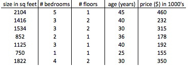
Let's take our previous housing data and add a few additional features:

From left to right, the corresponding variables would be x₁​​, x₂​​, x₃, x₄, and y. We use m to denote the number of training sets. Other definitions:

• n = number of features (e.g. x​​​₁​​ - x​₄​​)

• xⁱ​​ = input (features) of i​th​​ training example

• x​ₖ⁽ⁱ⁾ ​​ = value of features k in i​th training example

Though our previous hypothesis equation was defined as hₔ​​(x)=θ​₀ ​+θ₁x, with more than one feature, we update the equation as follows:

hₔ(x) = θ​₀ + θ₁x₁ + θ₂x₂ ​​+ ... + θ​ₙ​​x​ₙ​​, and for convenience of notation, define x​₀ = 1

Which means that we can define two matrices as follows:

\(\theta = \begin{bmatrix} \theta_0 \\ \theta_1 \\ \theta_2 \\ \theta_3 \\ \vdots \\ \theta_n \\ \end{bmatrix} x = \begin{bmatrix} x_0 \\ x_1 \\ x_2 \\ x_3 \\ \vdots \\ x_n \\ \end{bmatrix}\)

In this current form of n x 1 matrices, we can't calculate the hₔ​​(x) (remember, the inner dimensions, in this case 1, must match). The solution is as simple as doing a matrix transpose and then multiplying.

So, this:

\(h_\theta(x) = \theta_0 + \theta_1 x_1 + \theta_2 x_2 + ... + \theta_n x_n\)

can be rewritten as:

\(h_\theta(x) = \theta^Tx = \begin{bmatrix} \theta_0 & \theta_1 & \theta_2 & \theta_3 & \cdots & \theta_n \end{bmatrix} * \begin{bmatrix} x_0 \\ x_1 \\ x_2 \\ x_3 \\ \vdots \\ x_n \\ \end{bmatrix}\)

and we would end up with an n x 1 result vector. I thought this was one of the coolest things—being able to perform what would be an iterative calculation and do it in one go with a single matrix operation. This was where school-taught theory (which seemed to have no basis in practical work) actually made perfect sense for the problem at hand.

The equation for gradient descent for multiple features is:

\(\theta_j := \theta_j - \alpha\frac{1}{m}\sum_{i=1}^m(h_\theta(x^{(i)}) - y^{(i)})x_j^{(i)})\)

As you can imagine, however, given the varying scales in the universe of possible features for a given hypothesis (e.g. sqft, # of bedrooms, floors, etc.) plotting out the results will result in skewed shapes which will result in inefficient walking of gradients to local/global minima. So there are a couple techniques to make these more efficient:

• feature scaling: as the name implies, we perform some mean normalization on the inputs to make sure they are all on the same scale where −1 ≤ x​ₖ ≤ 1, etc. For example, for each given input, e.g.

• adjustment of learning rate: this is the α multiplicand in the gradient descent equation above. This will increase/decrease the rate at which we reach convergence. For sufficiently small α, J(θ) should decrease on every iteration. If α is too small, gradient descent can be slow to converge, requiring a very large number of iterations to obtain the solution, or if α is too large, J(θ) may not decrease on every iteration and, furthermore, may never converge. Rule of thumb for selecting α is to start from 0.0001 and increase by factors of 3: 0.0001, 0.0003, 0.01, 0.03, 01., 0.3, 1,...

That's enough for today. Next time, we'll go over polynomial regression for more sophisticated, non-linear hypotheses.