Rediscovering Math Through Machine Learning

The promise of AI has tantalized computer scientists and the general public for a long time, with general human intelligence out of grasp even still, however, modern advances in approaches to implementing machine learning algorithms coupled with a dramatic growth in computational capacity have yielded powerful tools to address discrete problem domains. What machine learning isn't, is trying to build human-level general intelligence into machines. Instead, as the name connotes, it's about creating programs that enable computers to use example data or past experience to solve a given, discrete, problem.

In order to pursue my interest in ML, I'm enrolled in Coursera's machine learning course taught by Stanford Adjunct Professor of Computer Science, Andrew Ng. The course is intended to be accessible to relative lay-people without any meaningful background in linear algebra or formal computer science. Normally, hearing the words "linear algebra" would make my eyes glaze over, but the math involved in the course is simplified, indeed accessible, and mostly pertaining to matrix operations which are pretty straightforward anyhow.

What surprised me was how interesting the math was and how we could apply it to solve computational problems. I suppose this is the difference between theory and applied math and it was striking to see how powerful and efficient certain mathematical operations could be in solving otherwise iterative computational problems.

In the course, we start with supervised learning where we supply attributes and expected results—in other words, for each data sample, the "right answer" is provided. This presents a regression problem where we predict real-valued output based on the supplied training data. So, given a training set, a learning algorithm, we create a hypothesis (h​ₔ​​) on the expected output based on a data point outside the sample, described by the following equation (when considering linear regression with a single variable/feature):

\(h_\theta(x) = \theta_0 + \theta_{1}x\)

where θ₀ ​​and θ₁x represent the training set parameters and xx represents the single feature input. In this form, this is a basic 1st-degree polynomial (linear) equation where θ₀​​ is the y-intercept and θ₁ is the slope.

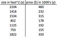
Here's an example data set of house size (x) to price (y) and the corresponding scatterplot:

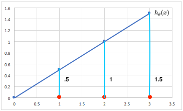
What we're trying to do is find the line that fits this data the best (linear regression). Using the h​ₔ​​(x) equation above and what we know about 1st-degree polynomial equations, we can observe the following given certain values of θ₀ and θ₁​​:

Where hₔ(x) = 0 + 0.5x (y-intercept 0, slope 0.5):

Where hₔ(x) = 1 + 0.5x (y-intercept 1, slope 0.5):

Now what we want to do with the sample housing data is fit a line do the data that minimizes the distance between the data points and the line describing our hypothesis. In other words, we want to choose θ₀​​ and θ₁​ so that our h​ₔ​​(x) is close to y for our training examples (x,y) so that we have something like this:

The "cost" of the hypothesis (our fitting equation) is the sum of the squared difference between the hypothesis (point on the line) and actual data point. So our goal is to determine the best values for θ​₀​ and θ₁ to minimize the cost, whereby we find the best fit for the training data and allowing us to confidently determine values outside of the training set.

We would therefore define the cost function as follows (where m is the number of sample data):

\(J(\theta_0,\theta_1) = \frac{1}{2m} \sum_{i=1}^m(h_\theta(x^{(i)}) - y^{(i)})^2\)

and our goal is to

\(\underset{\rm \theta_0,\theta_1}{\rm minimize} J(\theta_0, \theta_1)\)

and we graph the costs for various values of θ₁. Let's walk through an example where we assume all the data points are described by the function 0 + 0x, basically the x-axis:

We'd calculate the cost as follows (using the differences between the expected and actual values and ignoring the constant θ₀​ term):

\(J(\theta_1) = \frac{1}{2m}(.5^2 + 1^2 + 1.5^2)= \frac{1}{6} * 3.5 \approx .58\bar3 \)

This represents a single value of J(θ) which we graph along with various permutations of θ. Let's do this for a few more examples of θ​₁​​:

• θ₁​= .6, we calculate the cost against a line with slope of .6. This means our values are (1,.6), (2,1.2), (3,1.8) and the cost calculated as follows:

• θ₁ ​​= .9, values are (1,.9), (2,1.8), (3,2.7) and the cost as follows:

• θ₁ = .4, values are (1,.4), (2,.8), (3,1.2) and the cost as follows:

For θ₁​ ​= .5, the cost would obviously be 0.

As you can see, these points describe a parabola, on a graph with θ₁ on the x-axis and J(θ₁) on the y, with a global minima at θ₁ = .5, which is where the cost (J) of this function has been minimized.

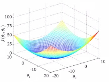
When we graph the individual parameters θ​₀​​​ and θ₁​​ against J(θ​₀​​​​​,θ₁​​), we get a contour plot/figure as follows:

I'll leave things at that for now and continue with the concept of gradient descent next time.